 GO Train acceleration analyzed by video
Introduction
It is well known that you can compare two successive images to find out how much objects moved between the images. I wanted to see if I record a train on video and infer its motion via algorithms. This analysis was all done at a distance, without touching the train or attaching any sensors onto it.
This idea led me on a journey of building a number of software tools:
- Image motion search in plain Java
- Matrix solving in Python and NumPy
- Time series derivatives and smoothing in Python and NumPy
- High-quality text rendering in Java
- FFmpeg command lines for video processing
Note: The source code posted on this page is very specialized to this project, and is only shown for reference. To use it for other purposes, adapting the code will require non-trivial expertise and effort.
Video
Graphs
 |
 |
 |
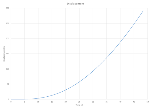
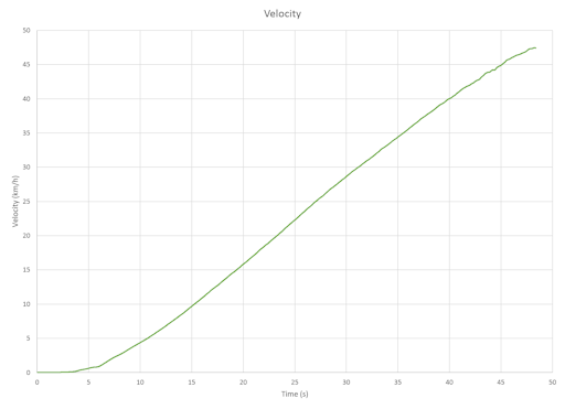
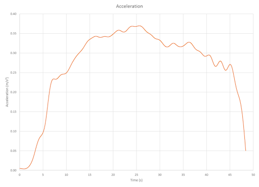
We can see that in 48 seconds, the train accelerated from a standstill to 48 km/h. For most of the time, the acceleration achieved by the train was about 0.33 m/s2.
Procedure
- Step 0: Video acquisition
-
I went out and personally filmed the video for the analysis. This ensured tight control over parameters such as lighting, perspective, lens choice, etc.
- Location: A grassy field 110 m west of Old Cummer GO Station
- Coordinates: 43.79348° N, 79.37301° W, 154 m
- Date and time: -Fri 15:41 UTC−4
- Camera: Canon EOS 6D
- Lens: Canon EF 100mm f/2.8 L macro IS USM
- Aperture: f/6.3
- Shutter: 1/1000 s (per frame)
- ISO: 200
- Codec: MPEG-4 AVC/H.264, all I-frames
- Resolution: 1280×720
- Frame rate: 59.94 Hz
Notes:
The macro lens was selected because of long focal length and low distortion. It would be bad to use a wide-angle lens to photograph the train because if the train was not perfectly perpendicular to the lens’s optical axis, then parts near the edge of the image frame become stretched. Secondly, this macro lens has low geometric distortion, whereas wide and medium lenses tend to have barrel distortion and telephoto lenses tend to have pincushion distortion. The lack of distortion means that anywhere in the image, the same pixel distance corresponds to the same real-world distance.
The camera was obviously mounted on a tripod. The lens’s image stabilization was disabled. This prevented drift and false compensation for no motion. But unfortunately there was some minute shaking due to the wind. In retrospect it might have been better to enable IS. You can see the effect of wind shake by staring at the power lines at the top part of the video.
The camera sensor is suboptimal for video recording. The Canon 6D does a poor job of vertical scaling, because it drops lines from the sensor instead of interpolating them properly. You can see this in the ugly jagged appearance of the power lines. Also, this camera forces the user to choose between 1280×720@60Hz or 1920×1080@30Hz recording. Other cameras can support 4K@60Hz resolution with no jaggies. In retrospect it would have been better to record at 1920×1080@30Hz because spatial resolution seems to be more important than temporal resolution in this analysis.
Manual exposure settings and white balance were used, thus keeping the exposure and colors constant throughout the entire video. The small aperture ensured a sharp image, and the short shutter speed (with the train conveniently facing the sun) ensured essentially no motion blur.
Judging by eye, the camera was pointed to the plane of the train as perpendicularly as possible, and the roll was made as horizontal as possible. Indeed, the motion analysis shows that the rotation error is only about 0.12°.
The train ran northbound on the Richmond Hill line, nominally arriving at Old Cummer at 15:37.
Result: MVI_22688.mov (673 MB, not published)
- Step 1: Convert to image frames
-
Using the versatile FFmpeg command line tool, the video file was converted to a sequence of BMP image frames, for easier consumption in later steps. Along the way, the unneeded top and bottom portions of the image were cropped away to save storage space.
Command: ffmpeg -i "MVI_22688.mov" -pix_fmt bgr24 -filter:v crop=1280:192:0:266 -start_number 0 "step1/%04d.bmp"
Result: 4088 BMP images (3.014 GB, not published)
Run time: ~10 seconds - Step 2: Trim, decimate, upsample
-
The beginning part of the video shows the train standing still, and the ending part shows the train gone from the scene. These are uninteresting and need to be discarded. The trimming is done at this stage instead of using FFmpeg, so that frame-accurate indexing is ensured. Analyzing the motion at the full 60 Hz frame rate would take too long and generate too much data, so I decided drop frames by 3×, resulting in a 20 Hz image sequence.
The upcoming motion analyzer was designed to search integer pixel displacements, because subpixel processing makes the program slower and more complex. However analyzing subpixel motion is desirable especially during the first few seconds when the train is moving slowly. So I chose to upsample all the frames by 4× using my high-quality sinc interpolation, and still running the dumb whole-pixel motion search. Finally, the pixel values were converted from gamma space to linear space, to make the image differencing less biased (not rigorously justified).
Source code: PreprocessFrames.java
Command: java PreprocessFrames step1/ step2/
Result: 971 BMP images (11.454 GB, not published)
Run time: ~3 minutes - Step 3: Motion search
-
The basic idea is to take some pair of image frames, crop a rectangle from the first image, find the best match in the second image, and record the spatial displacement. To start, we can do this for every adjacent pair of frames so that we get a sequence of displacements over time. In other words, we compute the displacement between frames 0 and 1, then 1 and 2, then 2 and 3, et cetera.
While this naive approach produces decent local information about the motion, it doesn’t necessarily yield good global information about the motion. For example if we want to find the displacement between frames 0 and 10, we can sum the 10 individual displacements to get an approximation of this value. But if we compare frames 0 and 10 directly, we might get a different number, and this number is more important than the small displacements calculated between adjacent frames. In fact, we want to calculate the displacement between every pair of frames as long as some portion of the train is present in both frames.
Another consideration is the speed of the motion search. Doing brute force comparisons of many subimages will take a long time, especially because the frames have been upsampled. Instead, we take advantage of the fact that the motion varies only a little from frame to frame. First we compute all the adjacent-frame displacements. After we compute the displacement between frames 0 and 1, we use this displacement as the estimate for the displacement between frames 1 and 2, and search only a limited number of neighboring candidates (such as within ±3 pixels of this value). Similarly, after we knew the displacement between frames 0 and 1, we double this amount to get an estimate for the displacement between frames 0 and 2, and search some neighboring candidates of this estimate.
All in all this procedure produces a large text file of about 100 000 lines, where each line says “From frame number i to frame number j, the best motion estimate is that the train moved (dx, dy) pixels”. For the particular input data and search configuration, this step took about 3 hours (multi-threaded) to run on my computer. The computation time can be reduced by reducing the frame rate, resolution, and search range.
Source code: FindMotionVectors.java
Command: java FindMotionVectors step2/ > step3.tsv
Result: step3.tsv (1402 KB)
Run time: ~3 hours - Step 4: Motion analysis
-
The result of the previous step is many thousands of observations that assert the train’s displacement between pairs of frames. We can put this data into a large system of linear equations and ask for a least-squares solution of it. Suppose we’re only interested in the x coordinate (the y coordinate will follow the same logic). We set up one variable per frame number, like x0, x1, ..., x999, each representing the global x displacement at that frame. Then for each line of the text file, we add an equation like xj − xi = dxi,j, which says “The x coordinate at frame j minus the x coordinate at frame i equals dxi,j”. One more constraint is added to fix the ambiguity in the solution, which is the equation x0 = 0. The matrix has as many rows as lines in the text file. All in all, the matrix’s dimensions are about 100 000 × 1000, takes about 1 GB of memory using float64, but is sparse because each row has only 3 non-zero entries.
Linear algebra seems to be easiest in Python with the NumPy library, so I switch languages because there doesn’t seem to be a convenient way to do linear algebra in Java. This step takes about 2 GB of memory and a minute to run, and the result is a small text file (~1000 lines) describing the best-fit displacement at each frame. Each line basically says, “At frame i, the train has moved (dx, dy) relative to frame 0 (which is defined as (0, 0)), as a best guess based on all of the available information from observations”.
Source code: fit-motion-displacements.py
Command: python fit-motion-displacements.py step3.tsv > step4.tsv
Result: step4.tsv (59 KB)
Run time: ~1 minute - Step 5: Motion postprocessing
-
The result the previous step is just a list of pixel displacements at each frame. First we need to convert these to numbers in real-world units. On the web, a diagram showing the dimensions of a GO Train passenger car can be readily found. The height of a rail car appears to be 651 pixels (in the 4× supersampled frames), thus the conversion factor is 1 pixel = 7.452 mm. We assume that the horizontal and vertical scales are equal (which requires the optics and sensor to be non-animorphic, and for the camera aiming to be perpendicular).
With the time series of displacement values, we are interested in calculating the velocity and the acceleration of the train as well. Not knowing any better, I took the naive approach of implementing finite differencing to calculate velocity and acceleration – namely I subtract two successive entries and divide the difference by the time step.
This simple method produced a mediocre graph for velocity, but a wild and unacceptably noisy graph for acceleration. Furthermore, I wanted to interpolate the motion analysis results at 20 Hz back to 60 Hz so that changing numbers can be drawn on every video frame. Thus I implemented a Gaussian convolution to smooth and interpolate the values, with hand-picked blur amounts depending on the data set in order to make it look nice.
In theory, the logic in this step could be appended to the end of step 4. But step 4 takes about a minute, whereas step 5 is instant. Step 5 requires trial and error, so it is best to make this a separate step in order to avoid recomputing the expensive part over and over again.
The finite differencing and the Gaussian smoothing that I used are not ideal. If I understood the math better, I would have used some kind of spline or regression to smooth the data and take derivatives of the smoothed displacement function.
Source code: derive-and-smooth-motion.py
Command: python derive-and-smooth-motion.py step4.tsv > step5.tsv
Result: step5.tsv (178 KB)
Run time: < 1 second - Step 6: Graphing
-
I took the result from step 5, fed the numbers into Microsoft Excel, customized the appearance of the graphs, and exported them to image files for publishing. Not much to say here, really. Other possible tools include LibreOffice Calc, gnuplot, Chart.js, Google chart tools, etc.
Result: See the “Graph” section near the top of the page.
- Step 7: Text overlay images
-
Using the sequence of numbers from step 5, I wrote a Java program to render some text to one transparent PNG image per video frame. The two special things about this program are that the text outlines are painted by brute force using a circular neighborhood filter, and the text is rendered without antialiasing at high resolution but then downsampled using my high-quality sinc resampler. This step takes a long time to generate the output because I chose to implement a high-quality renderer with simple logic. The time can be reduced by multi-threading, reducing the upsampling factor, or replacement with more efficient graphics algorithms.
Source code: RenderFrameTextOverlays.java
Command: java RenderFrameTextOverlays step5.tsv step7/
Result: 1451 PNG files (110 MB, not published)
Run time: ~3 hours - Step 8: Composite and re-encode
-
Finally, we trim the source video’s time range, overlay the appropriate text image on each video frame, and re-encode it for publishing. See the top of the page for the final output video.
Command: ffmpeg -ss 16.516 -t 53.0 -i "MVI_22688.mov" -r 59.94 -i "step7/%04d.png" -filter_complex "[0:0][1:0] overlay=eof_action=pass" -vcodec libx264 -profile:v main -g 200 -crf 20 -b:audio 192k step8.mp4
Result: step8.mp4 (42.1 MB, not published)
Run time: ~1 minute